


Login and Complete and Upload Excel Tasks (ATC)
Question Description
-
Discussion: Merging and Centering Cells (Due Wed., Feb. 5th)
We have learned a variety of tips you can use to create visually appealing tables in Excel, including applying table and cell styles and changing the size of rows and columns.Another helpful Excel tool is the ability to merge and center cells and to wrap text within a cell.
- Select the cells you wish to merge into one larger cell.
- Click “Merge & Center” from the “Alignment” group of the ribbon.
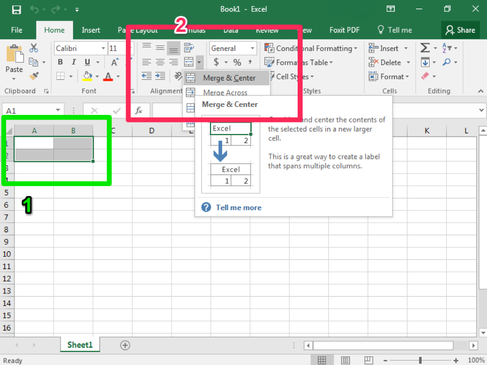
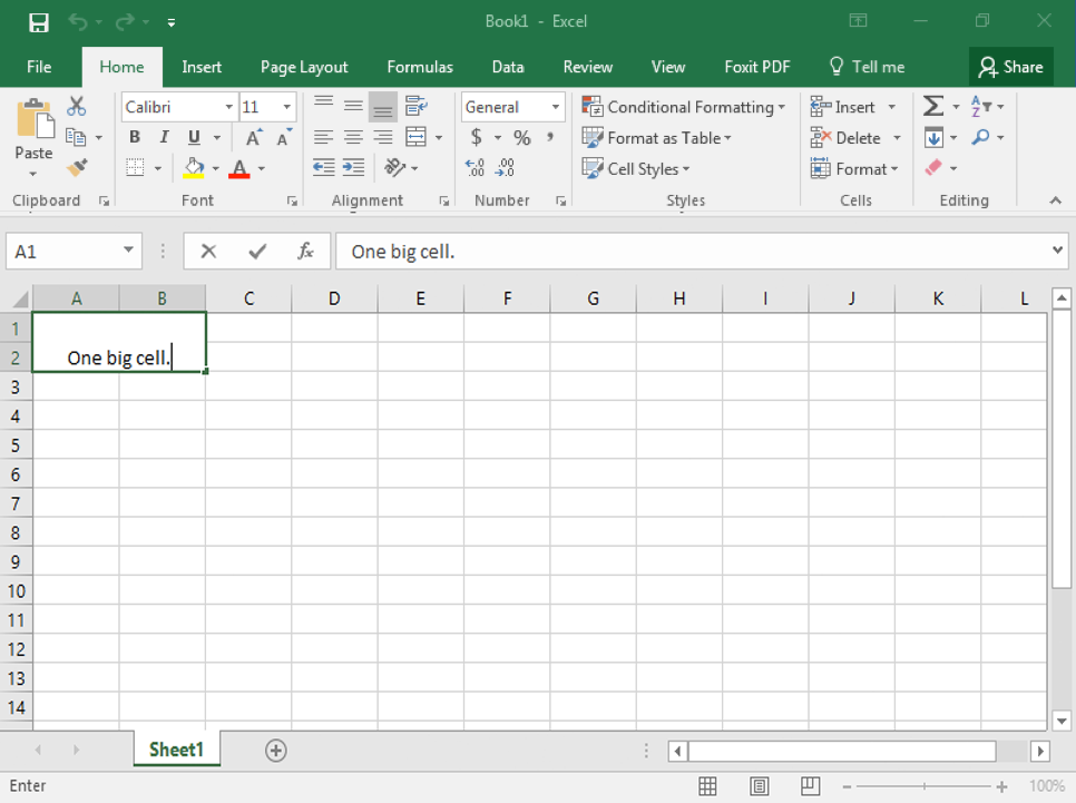
- When you type in this merged cell, the text will automatically be centered left to right in the cell.
 Now consider these questions: In what situations would this feature be useful? Would you ever use this feature? Why or why not?Share your opinions and post a reply response to two of your classmates.
Assignment: Organize Sales Data
For this assignment, you will manipulate an Excel worksheet to organize and display data about sales totals throughout a year.Download this Excel workbook. It already contains the data you need. Follow the directions, then submit your assignment. If you get stuck on a step, review this module and ask your classmates for help in the discussion forum.
- Open the workbook. Save it to the Rowan folder on your desktop as BA132_LastName_SalesData.xlsx, replacing “LastName” with your own last name. (Example: BA132_Hywater_SalesData) It is a good idea to save your work periodically.
- Format the data as a table with the name of the months and sales total as headers. You may use any table style you like.

- Change the cell format so that all the sales totals display as currency with a dollar sign and two decimal places.

- Indicate that the data for June and October needs to be verified by applying a different cell style to those cells.

- AutoFit the column width.

- AutoSum the total sales for the year.

- Save your work and submit the workbook to Blackboard.

MS Excel, Pt 2 PowerPoint
Assignment: Analyze Yearly Trends
In this assignment, we will pull together everything you have learned about Excel to analyze trends in sales data over several years.To complete this assignment, you will need the assignment you completed last module that you saved as BA132_LastName_SalesData.xlsx (or you can download the original assignment here) and a new workbook you can download here. Follow the directions, then submit your assignment. If you get stuck on a step, review this module and ask your classmates for help in the discussion forum.
- Open both workbooks. Save the new Module 7 file to the Rowan folder on your desktop as BA132_LastName_YearlyTrends.xlsx, replacing “LastName” with your own last name. (Example: BA132_Hywater_Memo) It is a good idea to save your work periodically.
- First, we need to combine the information into a single workbook. Add a new worksheet to the Module 7 file and copy the table from the Module 6 assignment to that new tab. Name the new tab “2014”. Be sure to set the number type to currency.

- For each individual year of data, sort the sales total “Z to A” so that the month with the highest sales is at the top. When you chose the “Sort” option, be sure to “Expand the Selection.” That will make sure that the months change as well. The screenshot below shows you only what 2012 should look like, but when you finish you should see October as the highest in 2012, August for 2013, and May for 2014.

- Add another new worksheet. Now we want to set up the spacing for the table we are about to make. Merge the 1 and 2 cells of column A, B, C, D, and E individually (so A1 and A2 merge, B1 and B2 merge, etc). Then name the cells as shown in the list below and center the text in those cells.
A = Month
B = 2012 Sales
C = 2013 Sales
D = 2014 Sales
E = Monthly Trends
- Copy the following columns of data over in order: “2012 Sales Total,” “2013 Sales Total,” and “2014 Sales Total.” Remember, you can just copy and paste each column in order, using the columns you have already labeled. When you autofit the column to the data width, your header cells will change.

- Now apply conditional formatting to your sales data to highlight any month with a value less than $4,000.

- Next, in the ‘Monthly Trends’ column, create a sparkline that shows performance for that month over the three years. Remember, after you create the first sparkline in January, you can just copy and paste into the other cells.

- Finally, create a clustered column chart of your data.

- Save your work and submit it to Blackboard.
Have a similar assignment? "Place an order for your assignment and have exceptional work written by our team of experts, guaranteeing you A results."